Geospatial Analysis is the catch-phrase of GIS maps and statistical investigations of data scattered with a reference to ‘place’. It is linkages found based on where and why something happens. Geospatial Analyses are conducted, normally, in GIS programs. Because technology has multiplied our abilities to overlay data as spatial references, we are able to discover new possibilities.
GIS maps have been considered “pretty pictures” for centuries. But now, we consider them virtual representations of the data seated inside. In FRASS, we use those hidden data linkages to discover new management possibilities. In the process, we discover hidden value to be revealed for our clients.
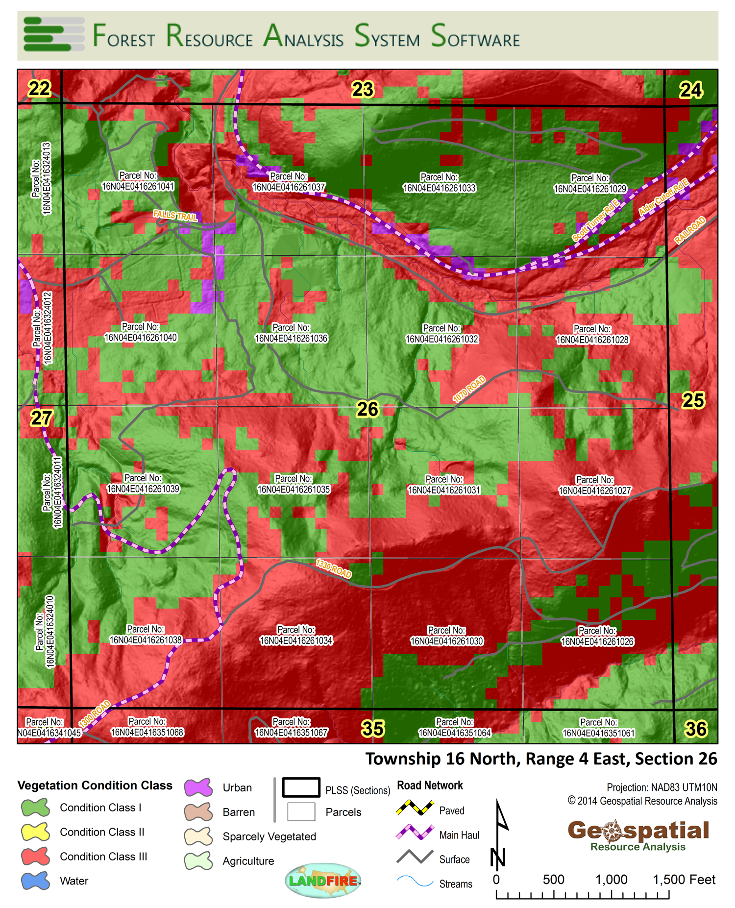
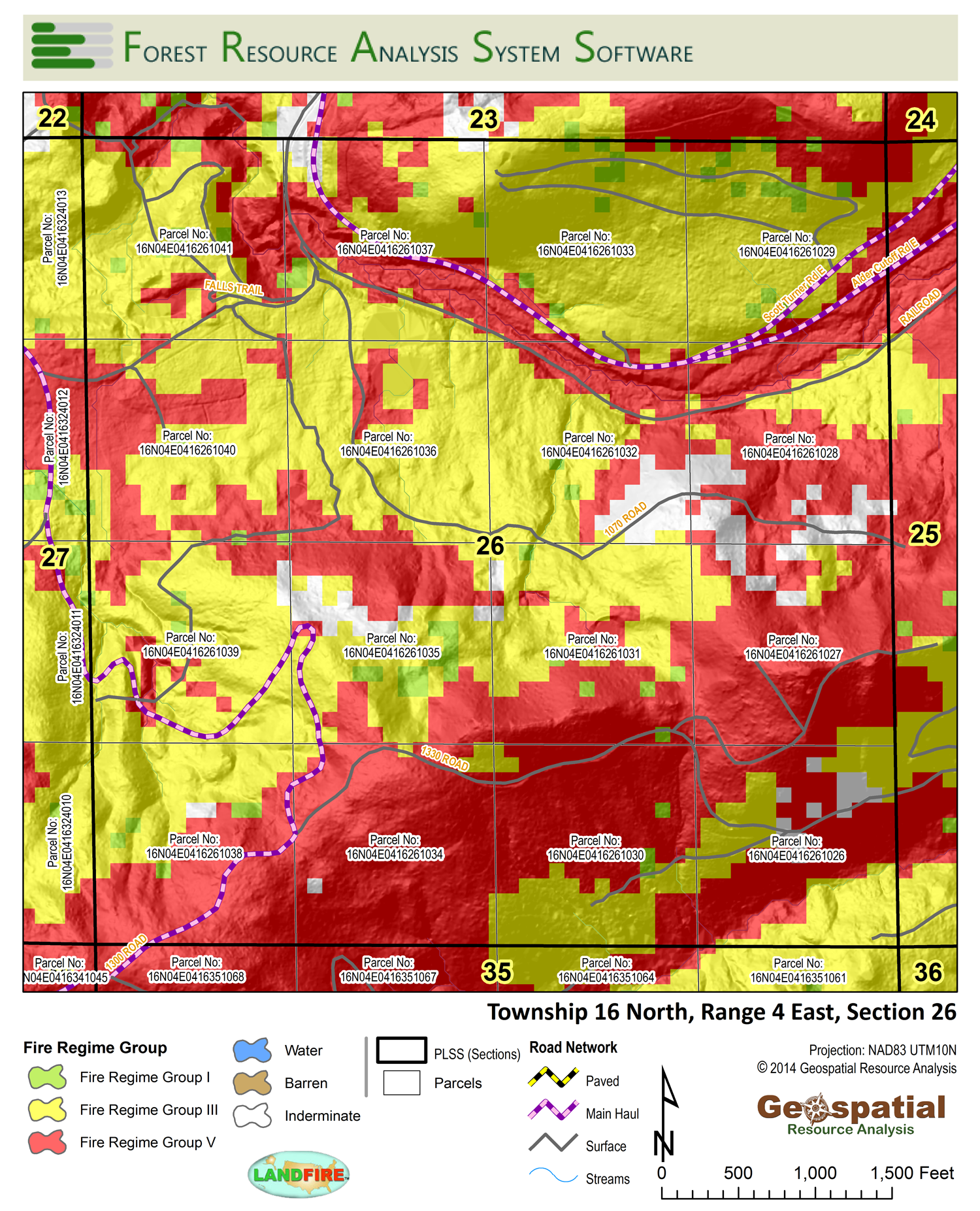
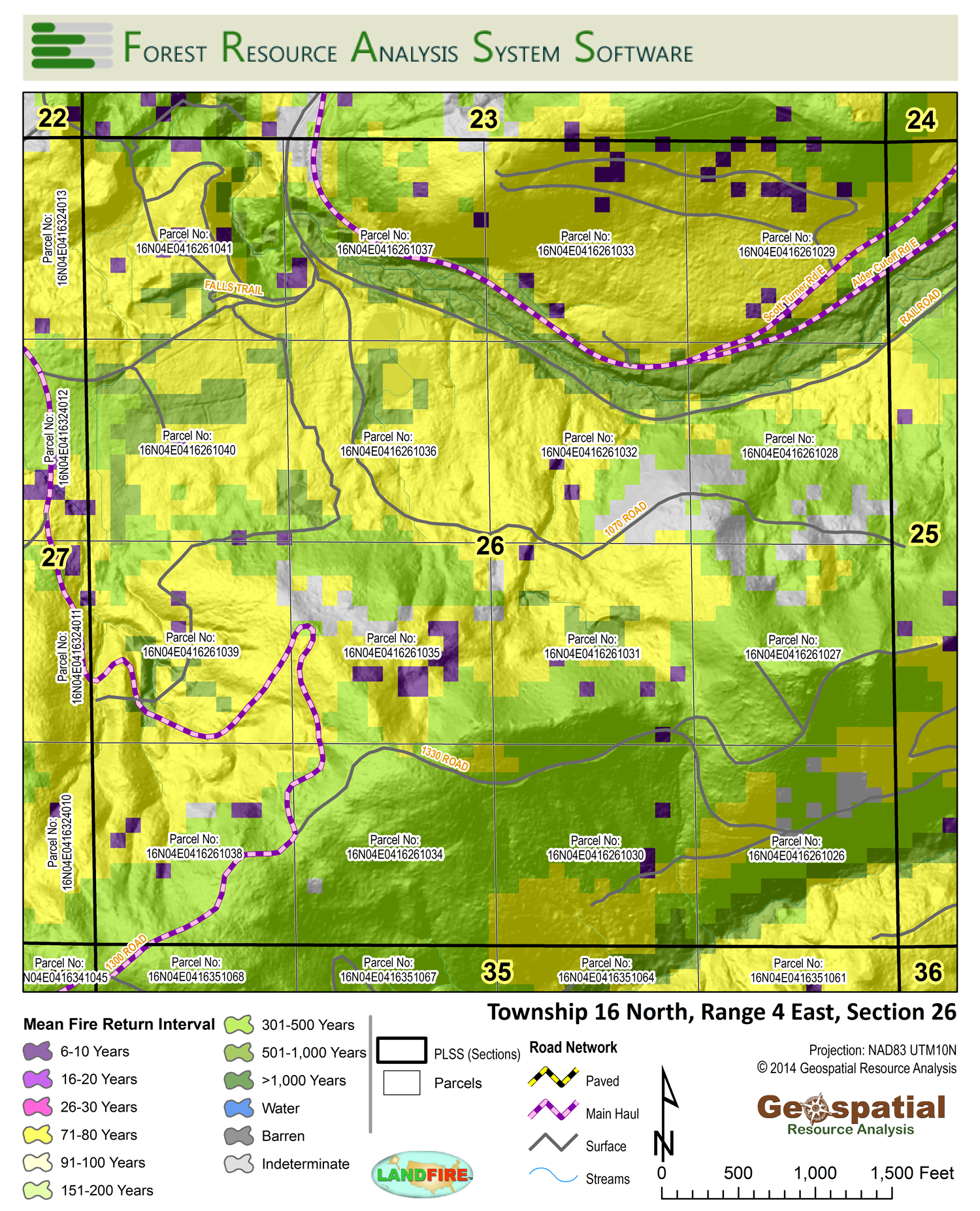
GIS Maps give a visual foundation to spatial data
Metsker Maps
As recently as 1970, forestland management offices, county assessors, and real estate offices were stocked with Metsker Maps. These were the lands they managed, or sought to manage, and they needed reference to ‘place’. Maps were a foundation of “spatial acuity” – use them when you need to know where it is.
USGS Maps
By 1985, the United States Geological Survey (USGS) had produced color maps of most lands in the USA. These maps were put to operational scales showing detail at 1:12,000. Most displayed the legal land survey leading to section, township, and range corners and boundaries with section numbers displayed. They drew topographic lines across the landscape labeled every 20 feet of elevation change. Roads and road classes, streams, and lakes were mapped. These USGS color maps took position as the tool used by every natural resource manager. Data became a part of map images. It stayed in this ‘preferred position‘ as it totally replaced Metsker Maps in management offices.
Geospatial Analysis
Geographic Information System (GIS) computer programs began to take interest of natural resource management offices soon after mainframe computers were introduced. Operationally, analysts could create maps using data about their properties. It became an attractive addition to the land management virtual tool arsenal. However, by 1990, GIS maps generated in local offices provided only a thin map product. These were compared with the attractive USGS maps people were accustomed to. It was a time when GIS mapping was still anchored to users on mainframe computer systems.
This changed by mid-1990 as RAM memory and hard-drive storage capacity boosted the capacity of PC users. Network systems facilitated user-data-sharing. Two public domain GIS systems were developed in the 1970 and 80s:
- Map Overlay and Statistical System (MOSS GIS), and
- Geographic Resources Analysis Support System (GRASS GIS).
They each made the migration to the PC, but today it is GRASS GIS which gains interest. GRASS is most attractive because of its ability to analyze raster and vector data. It is licensed under the GNU General Public License (GPL). The software works on Windows, Mac OSX, and Linux computer operating systems. Did we mention, “it is Free-Ware“?
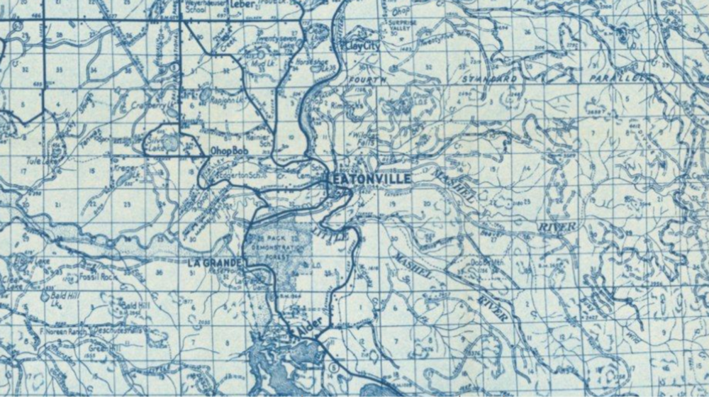
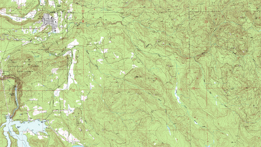
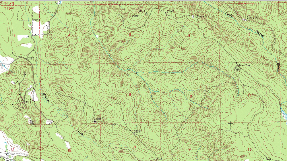
[Above] Metsker Map of Pierce County, Washington 1970, USGS Topographic Map of Eatonville, Washington 1990, USGS Topographic map of Pack Forest, 1:12,000 1997.
ESRI ArcGIS
Environmental Systems Research Institute (ESRI), made transition of software programs to migrate from the mainframe computer infrastructure to PCs. Eventually ESRI eclipsed others for the market-share of GIS globally. The capacity and breadth of the software has been endorsed by governments and universities insuring its market dominance. Known today only as ‘ESRI’, it has offices globally located where training programs and conferences insure its position as leaders in GIS analysis and programming.
College and University training programs in natural resources have embraced geospatial analysis programs. This extends far beyond just being part of introductory classes. GIS forms a key component of forestry, wildlife, geology, and fisheries degree programs. Graduate degrees are offered to expand the research in geospatial analysis, usually using ESRI GIS programs (ArcGIS or ArcMAP).
ESRI made a strong business decision when they made the ArcGIS program available to colleges and universities without charge. By making the software ‘free’ to these users, they insured a solid footing in the businesses the students landed with. Businesses must purchase licenses from ESRI for each user. But new hires come as trained ESRI Software users. These employees know how to integrate their vector and raster data efficiently. Businesses consider the software cost justifies the purchase, because their people know how to use it.
GIS Unites Spatial Data with Visual Acuity

The theme ‘maps convey visual data’ is something we take seriously at D&D Larix. Within the context of forestland resource GIS data accumulation, we assemble powerful core information:
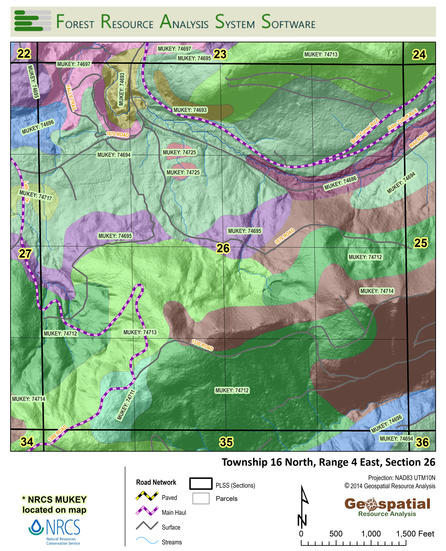
- soils,
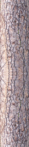
- aerial imagery,
- remote sensing imagery,
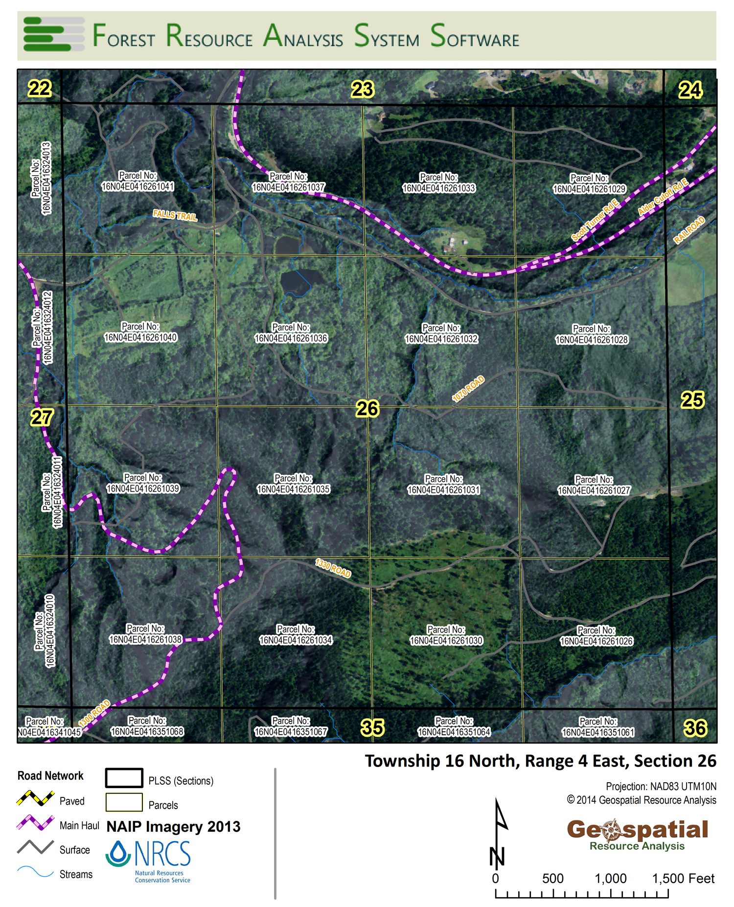
- digital elevation models,
- streams,
- hyporheic water flow channels,
- roads,
- bridges and
- culverts
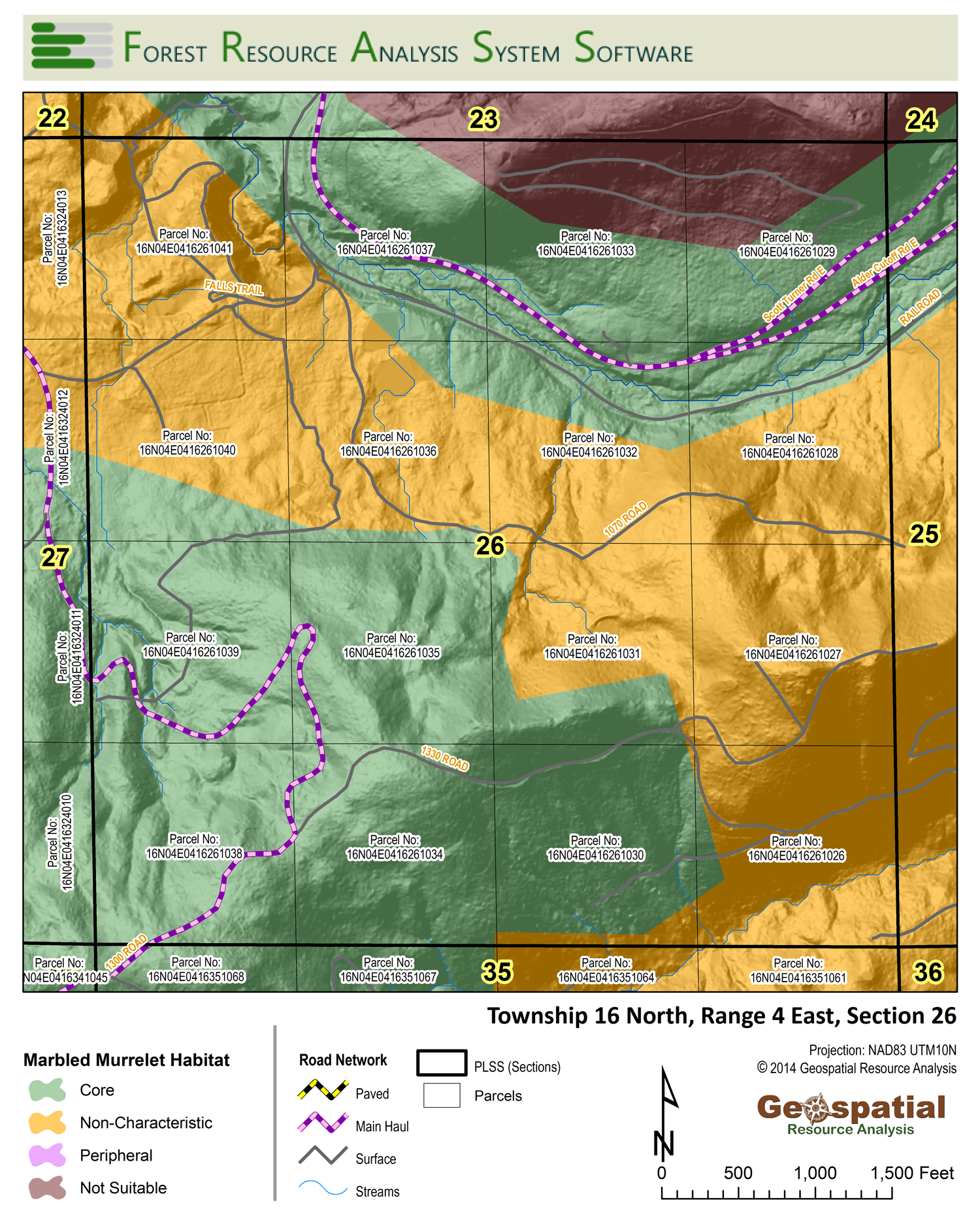
- threatened, endangered, sensitive species habitat range,
- anadromous fisheries habitat,
- timber stand boundaries.
These tools deepen land management decision making criteria. “Too much data” often causes people to shy away from seeking it. But when it is needed, more data can lead to better decisions. Here is where we make it happen.
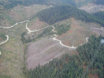
Do you see the hyporheic zone in the photo shown here? We find them from satellite imagery combined with some physical site characteristic data. Maybe you need to start by learning what a ‘hyporheic zone‘ is? These are important to support aquatic systems and water quality across the landscape.
Extending Your Reach
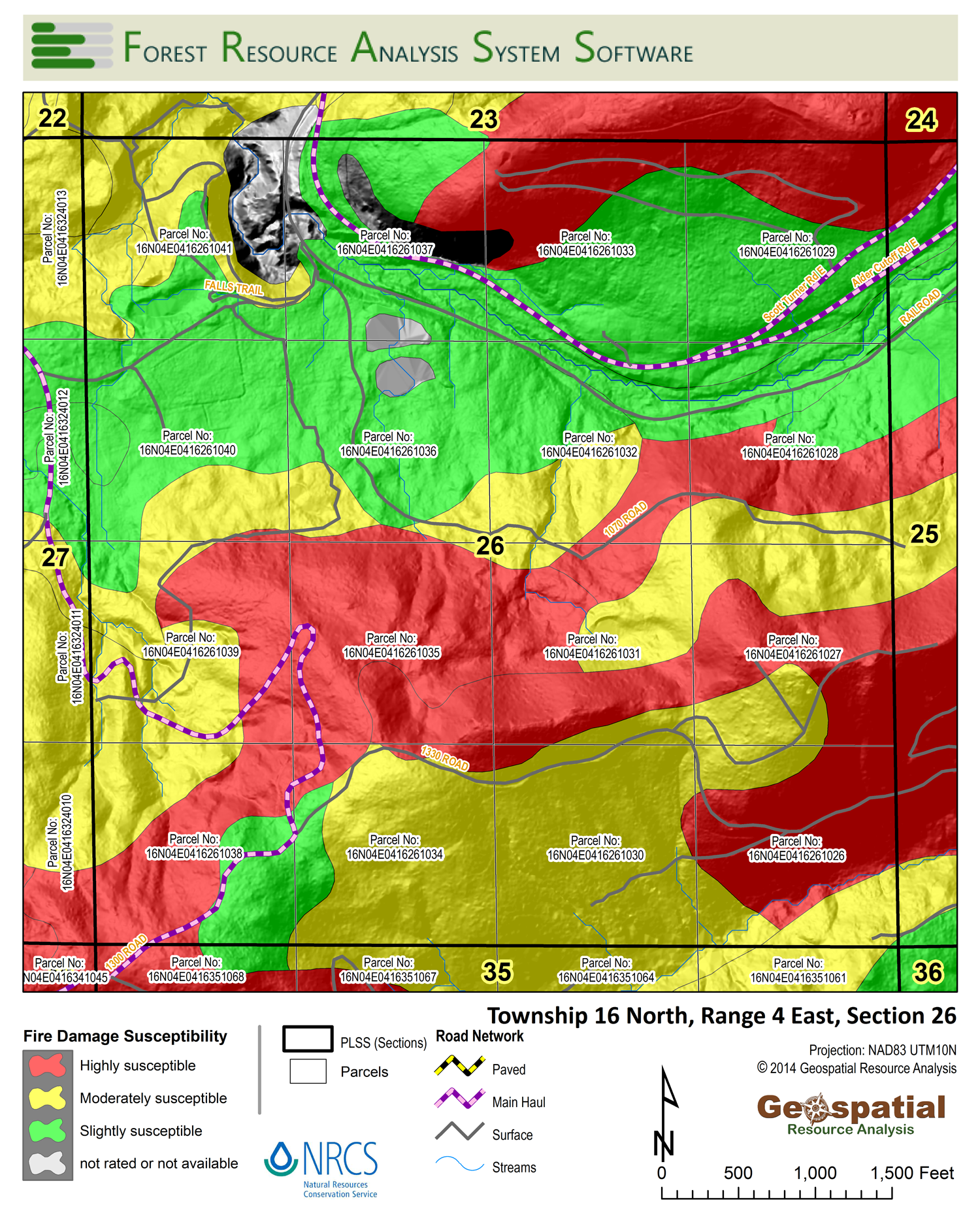
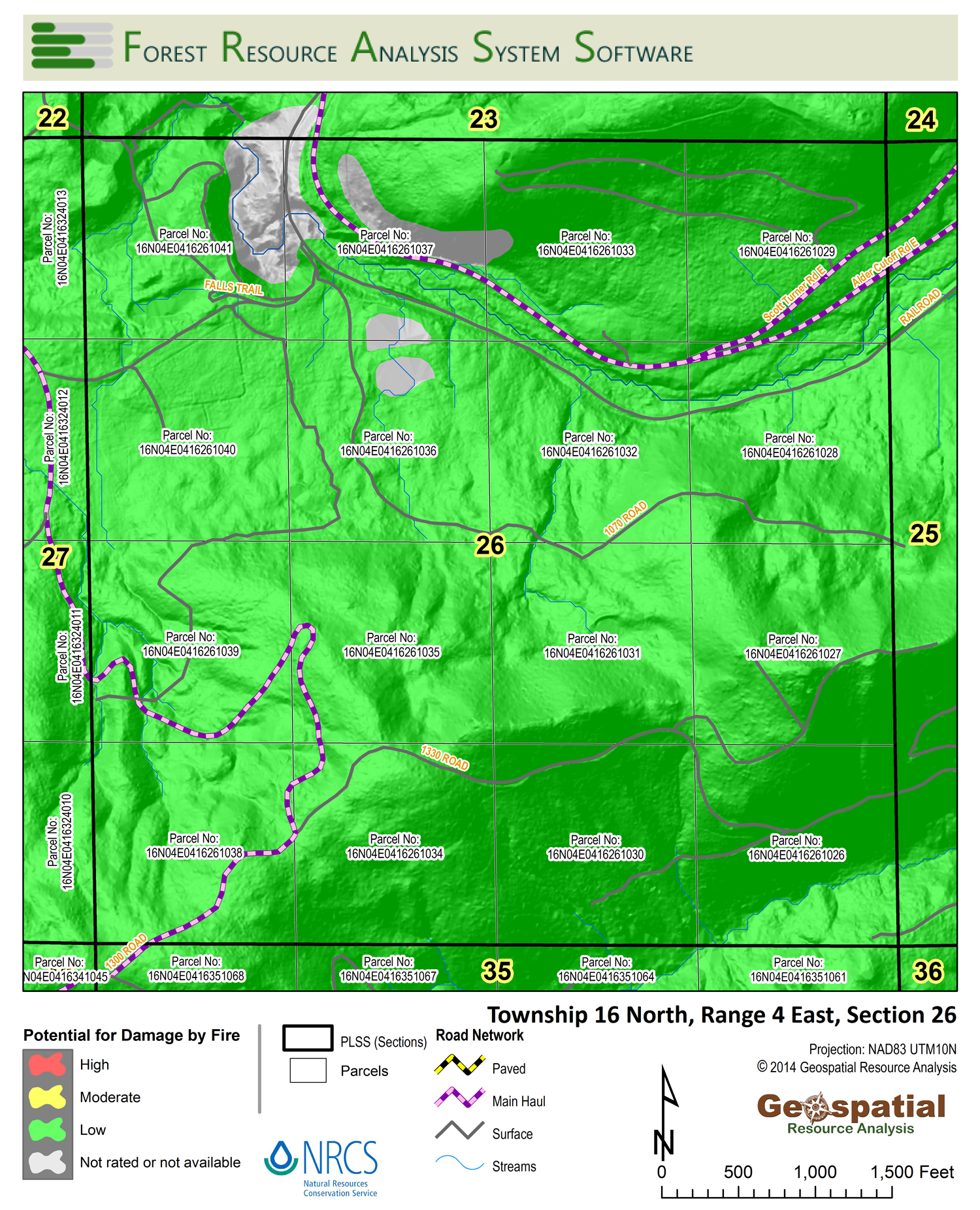
These data broaden understandings to derive links to wildlife habitat, fisheries, and natural hazard risks (wildfire, landslide, and flood). These provide resource managers a broad spectrum of management considerations. This means that while we may collect data for forest management purposes, we might expose other important attributes.
GIS has taken the position of a tool most all natural resource managers rely on daily. These data serve the resource manager as an X-Ray serves the medical service provider. We can visualize what is taking place on the land, under it, and around all we do.
In the USA, much of the vector and raster data we rely on is provided by federal agencies to all users, free-of-charge. Many groups develop additional data, and those are also commonly provided without charge to users. These data have become a core for land managers to accumulate and use. They are used to make more specific and accurate land management decisions.
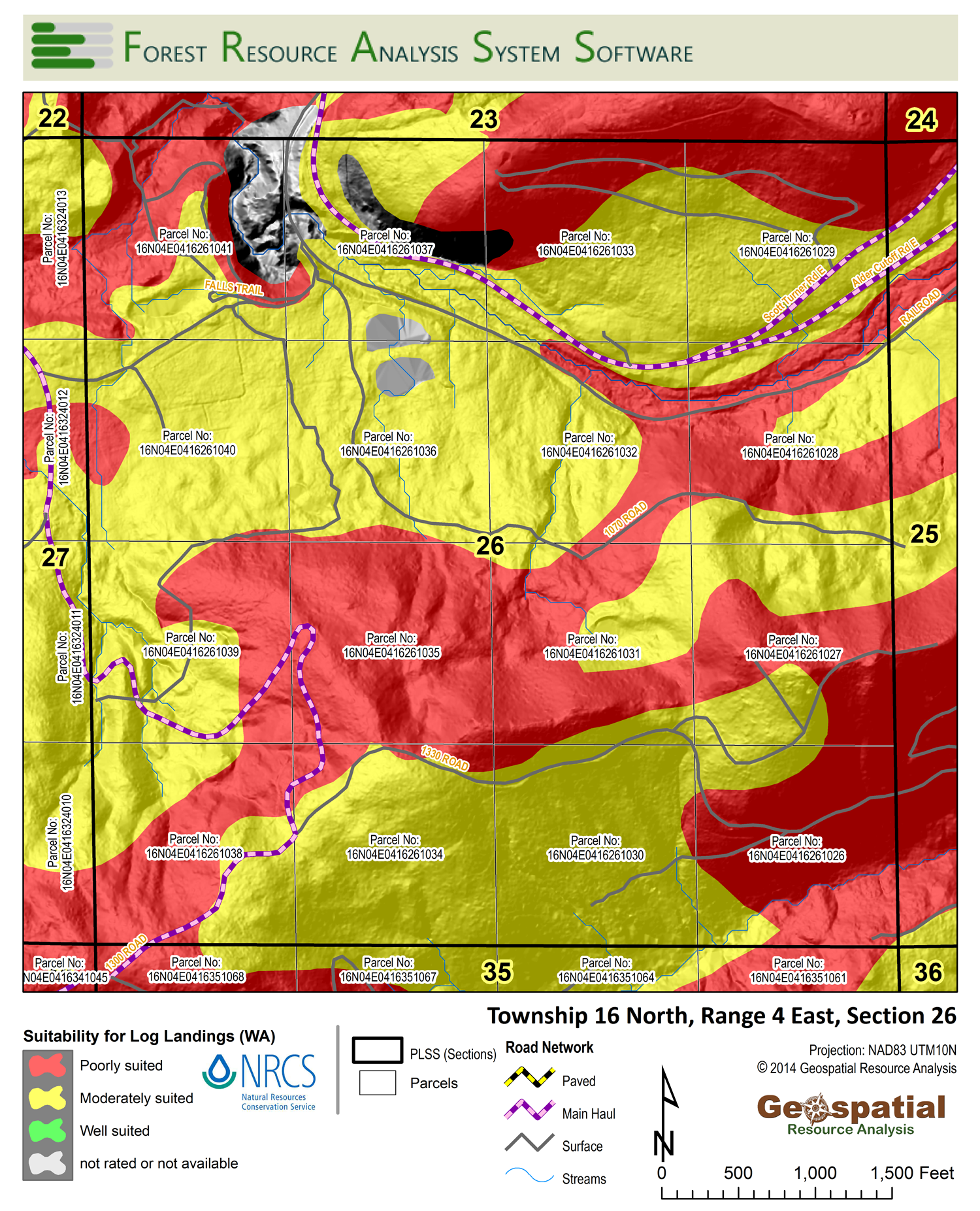
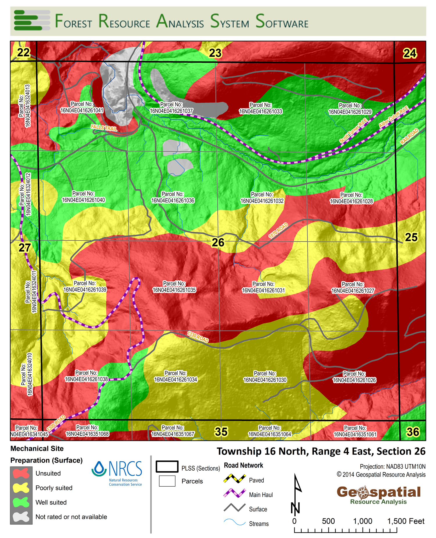
At Forest Econometrics (D&D Larix), we recognize that forestland owners possess much of the data we use in the FRASS Platform. It is data specific to the land being managed. We use the insights it provides, such as site suitability to road building or log landing construction. The soil survey data provides these data, and more, in free-to-use GIS data. Other data include records to discover the travel distances from log landings to log buyers who purchase the timber harvested. GIS data gives insights to juxtaposition between timber stands scheduled for harvest within temporal limits. That means “don’t clearcut in side-by-side timber stands for at least 5 years”.
Sometimes, we do what is “good”, as opposed to doing only what is “allowed”.
Deriving Data
Oftentimes, GIS data summarizes things we can see or measure on the land. This is how soil data are created, or a road position is mapped. Using GIS we extend these analyses to use “measured” attributes to create new data layers. This happens when Digital Elevation Models (DEM) are used to define the stream network. This is an encapsulated feature of geo-statistics to use the shape of the earth’s surface to discover stream placement in spatial terms. From this approach we extend it to define associated information:
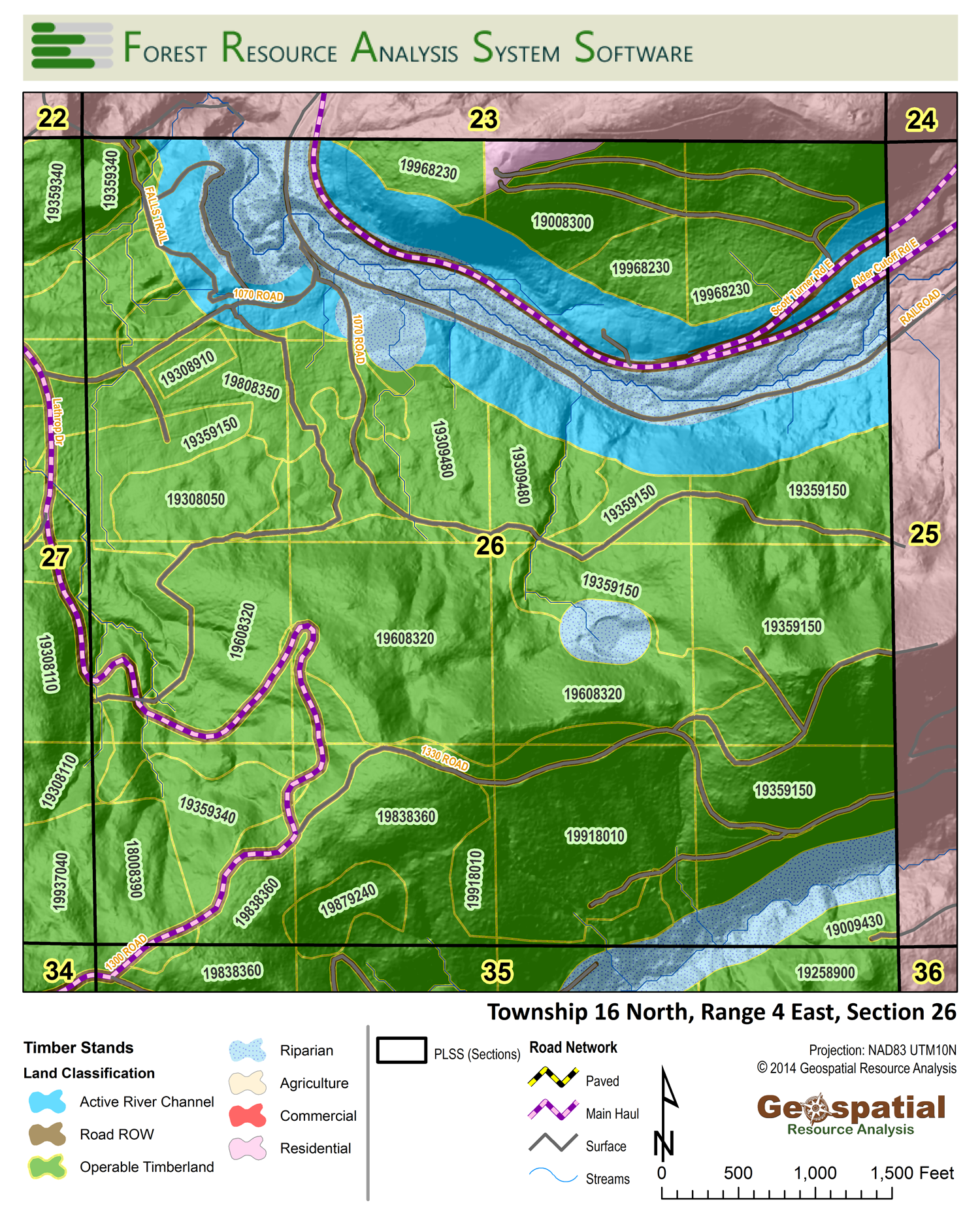
- active channel,
- aquatic lands,
- floodplains, and
- riparian zone.
Each segment is increasingly broader than the previous. A riparian zone is often defined administratively. This approach fails to make the stream-side relative width to the other segments definitive. The active channel and aquatic lands (1) and (2) – both represent property excluded from growing commercial timber. Both areas support an active aquatic process. These segments are mapped but not included in the operable timber growing lands of each timber stand.
Riparian zones are often described administratively (by state/province or federal regulations). This removes the trees from commercial harvest considerations, at least in the short-term. Depending on the interpretation of riparian zone’s administrative limitations, the lands may be completely removed from timber production. Trees may be administratively removed from even-aged management techniques. This approach favors of a single-tree removal, or green-tree retention strategies. This hopes to achieve a target tree density for the dependent stream.
Make Your Data Actionable
Over time, the riparian zone trees may be available for harvest through uneven-aged management techniques. It is critical to precisely identify the area and location of aquatic zones for sustaining a forested wildlife habitat. Maintaining an active forest Growth & Yield profile for those lands is critical. Mapping those areas makes the data actionable. This is important to articulate the wildlife habitat maintained and the merchandized timber characteristics through time.
Technological advances in geospatial analysis data has greatly expanded. The USGS announced the launch of Landsat 8 OLI (Operational Land Imager) and TIRS (Thermal Infrared Sensor) in 2013. These data, released free of charge to users, enables multi-spectral imagery analysis on lands around the world. Unlike the spatial resolution of previous Landsat satellites, Landsat 8 reveals scenes at 15 meter resolution. These scenes are updated on a 16-day repeat cycle.
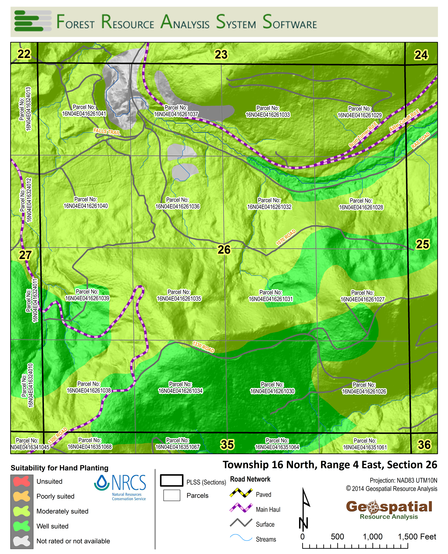
Physical site characteristics are documented, then promoted to parcel analysis in a mapping format. FRASS takes this to the next level when tabular summaries are used to extend their importance as they are associated with other data. These are valuable findings revealed through geospatial analysis and delivered to forestland management organizations using FRASS.
Stream layers and aquatic zones are examples of data findings revealed through GIS and geospatial analysis. There are so many more valuable attributes to discover. An active FRASS Platform for your operation is an important step to discover value in your operation’s data. Now, we take the next step, together.
GIS Data: its more than just shapefiles
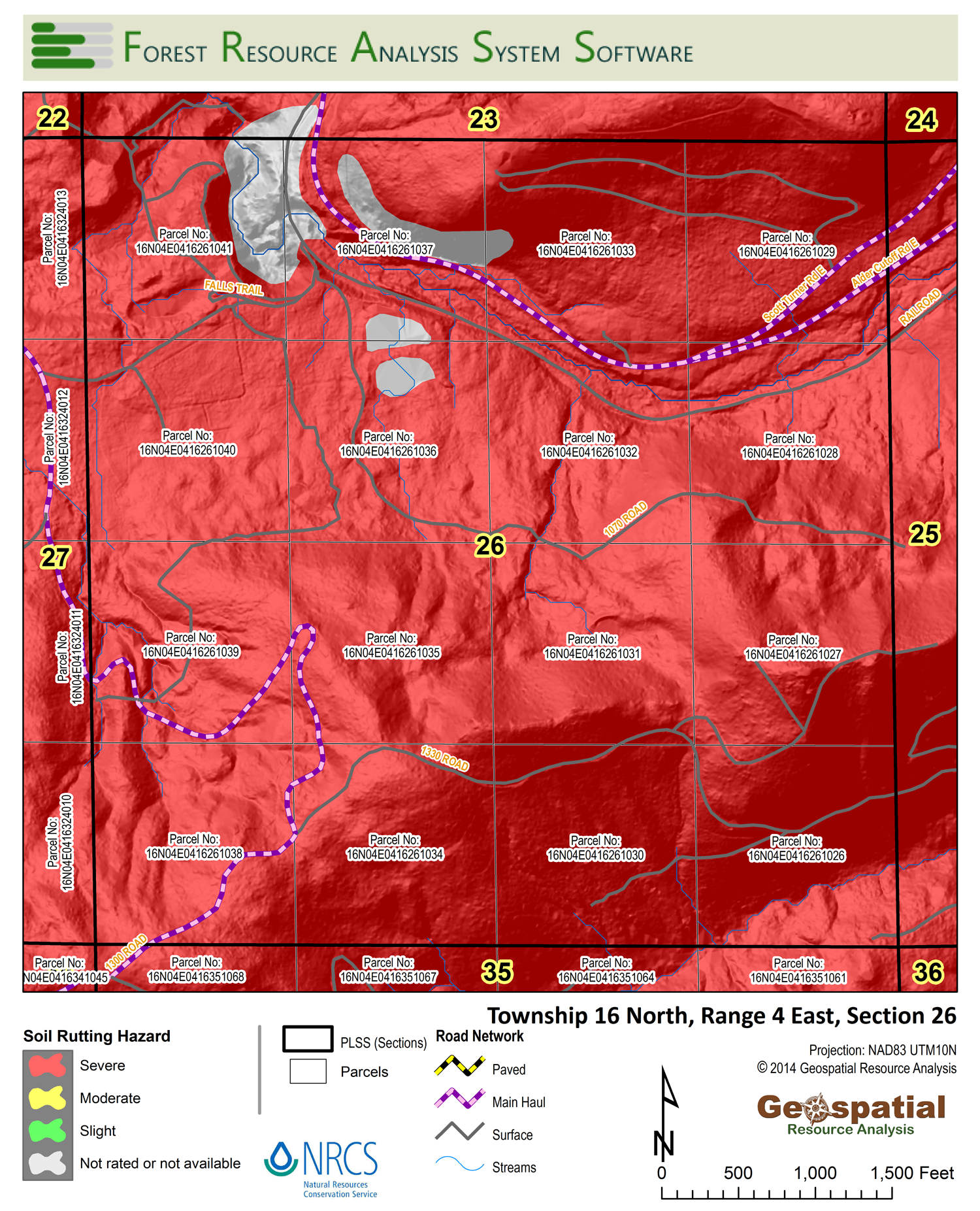
GIS data are stored in databases as a combination of spatial and tabular layers. Maps allow us to visualize spatial relationships within an intermix of physical land resource characteristics. These need to be seen and interpreted within specific contexts. Maps give us quick recognition of, for instance, the cost of building a new road. When neighboring properties do not have roads either, costs increase. We use the same relationships to consider the placement of log landings in response to limiting soil characteristics.
We treat maps as a visual data
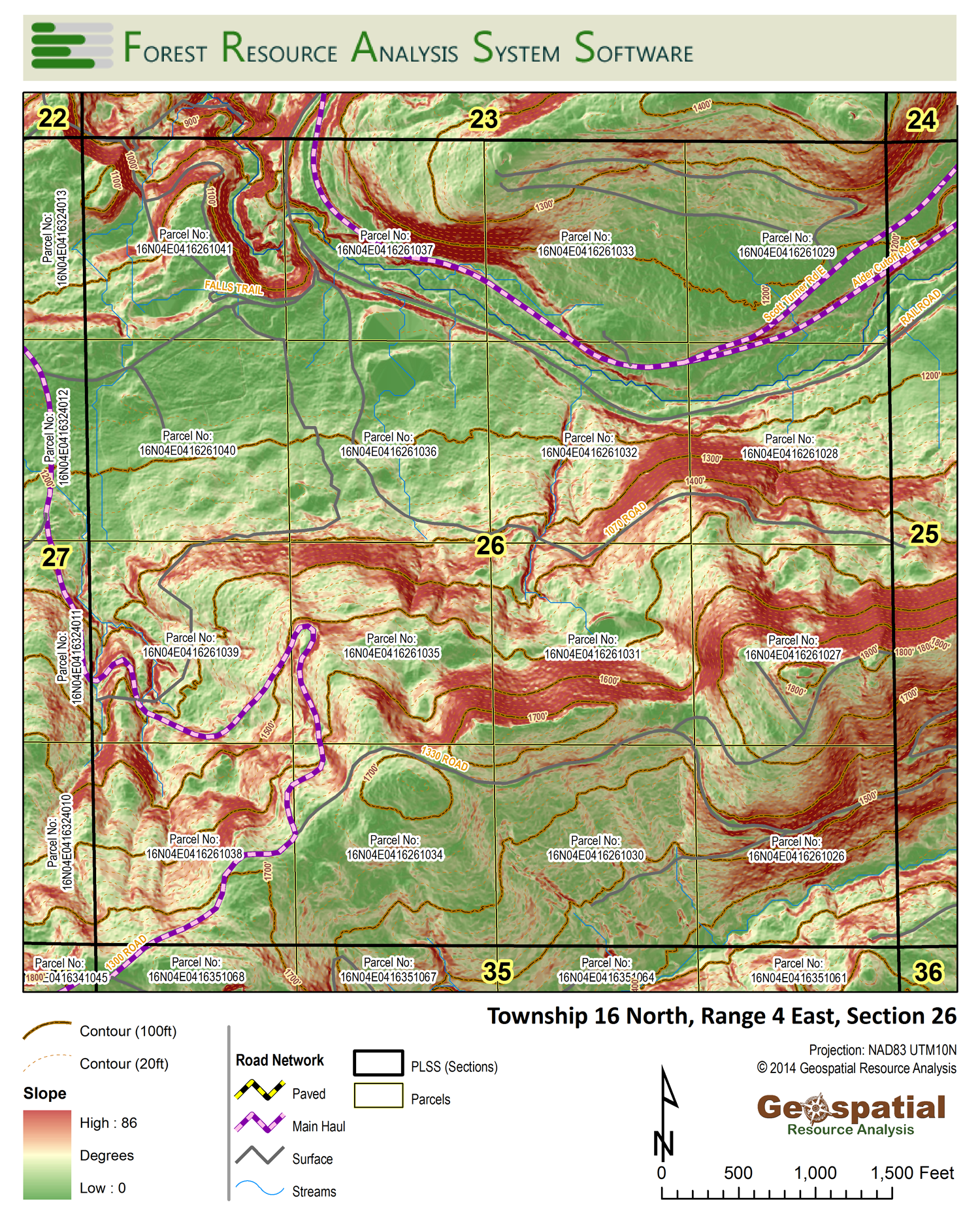
Tabular parcel data provide mountains of information. Spatial data have been translated into tables for each parcel separately to summarize its variable attributes. These values are compressed into content-charged data packages for the practical implementation by a landowner or manager alike. By summarizing these data blocks for each timber stand, we create easy-to-understand tools for highly specified analytical solutions.
Derived Geospatial Analysis Data
 One example of the advances in derived GIS data comes through Digital Elevation Models (DEM) analysis. By combining accurate elevation and topography data we drill into road network data. The science of land topography excelled to cover much of North America with 10 meter DEM. More recently, LiDAR flights have expressed the ability to display these same areas at 1 meter resolution. This creates a higher level of precision for further analyses.
For instance, we map roads while using 1-meter resolution LiDAR topographic maps to pinpoint road boundaries. Although we map roads as lines, they represent a polygon of area that is not otherwise available for growing trees. Roads represent non-operable lands to grow trees. Astute forestland valuation approaches will remove these areas from productive land categories, before seeking asset value.
A buffer around each road is determined to account for non-operable land. These areas are not available for growing timber or supporting wildlife habitat. Those areas are removed from the productive timberland base.
We have taken this approach to the next analysis level. Roads on a map are lines without slope – flat roads?. Most forest roads travel up the hill and down again. By using the high resolution LiDAR DEM data, we calculate road segment lengths as slope distances. This provides accurate travel distances, important for determining log trucking costs.
A River Runs Through Data as well
We use a similar approach when dealing with streams as they cross through a timber stand and a parcel area. Streams represent a complex meandering grid of aquatic flows of certain width. As an open road is associated with physical removal of timber growing lands, so do segments of the stream network. Trees growing in a river, stay in the river. Do not harvest trees that are part of the active channel network – fisheries habitat need those stems to stay put. Define the active channel and fish habitat can be protected.
Do you need GIS data created or analyzed on your property?
You need it to make your FRASS Platform operational. We can help you make it all.
Resource Analysis Specialists
We have worked with GIS staff who are tasked with responsibility to ‘map’ their organization’s properties. Most often this is done for specific purposes like forestry, fisheries, human habitation locations, or just infrastructure. Their GIS themes have mostly been well developed. But linkages to other data have often been scant. This is where our unique possession of data and analysis skills have been brought to task for our clients.
In some cases, we were asked to develop data the client did not have access to. We then unite the different mapping systems into one holistic unit. Often this was in the form of re-projecting spatial data references into one unified projection. These terms may seem foreign to the non-GIS specialist. But to those who have failed to get images to “match” on the screen will know what this is about.
Other instances have been built around data analysis from a few or many associated layers. We use these to develop derivative data layers of spatial analysis results. Visitors can scroll through the Resource Analysis web domain, in the Geospatial menu area. Explore some of the analyses we build from natural resources data.
In the Spatial Analysis, sub-link on that site, you will read about satellite data we analyze. The USGS LANDSAT 8 OLI satellite imagery is used to slice infrared and near-infrared layers. It reveals the discovery of sub-surface water content and mineral presence in exposed soils. Using these data, vegetative structural index, and even a ‘free to grow’ measure of tree growth conditions is displayed. These are combined with terrestrial GPS data layers, aerial imagery and management conditions known to the forestland owner.
This is how we deliver management insights to the forestland resource you already know. Now, you get to know those lands better.
Making Data Where None Existed
A project we completed in 2008 involved applying these skills to southeast Alaska. The project extended from Skagway in the north, to Craig on Prince of Wales Island in the south. The land area is about 49 million acres (19.8 million hectares). Using the 30m DEM data collected by the USGS, we created a GIS vector drainage layer. All stream classes were assigned a Shreve Stream Class. These data connected forest management activities with anadromous fisheries habitat.
We used satellite imagery to discover and map roads, stream crossings (bridges, culverts, and splash-crossings). We used the satellite imagery infrared slices to identify human habitation structures, paved roads, and persistent ice formations.
The Alaska region in 2008 was missing detailed imagery much of the continental US has benefited from: NAIP aerial imagery. By using the spectral imagery of the LANDSAT satellite, we were able to create a complete imagery mosaic. It was displayed as 15-meter resolution natural-color imagery for the region. These layers provided a previously unavailable “natural color aerial imagery-like scene” of SE Alaska. They made it possible to map timber stand boundaries, riparian zones, and road infrastructure components. It led to our creation and verification of a forest tree-species site index layer. This layer covered all of the timber lands of this region.
All geospatial data we created for our client was delivered to them as the project progressed. It enabled the development and deployment of their FRASS Platform.
This is what we do.